Network Traffic Analysis
Abstract
There is news about network infiltration every few weeks and the rate of the intrusion seems to be growing. No organization, big or small, is immune to this. While few breaches like uber, sony, yahoo and equifax get lot of press coverage, most of them go unnoticed in the mainstream. There are many instances where organization are unaware that their network has been compromised for a very long time. As complexity of software increases, there is increased attack surface for an adversary trying to infiltrate. And the attack only get better, for example, mirai botnet taking down dyndns using IoT devices seemed like a big deal but now there is reaper building larger army of botnets.
Network of any organization are build on hundreds of such softwares. The complexity of any network increasing with each passing day and every device imaginable seems to be running on of those complex software. Keeping all those software from routers and switches to television and cameras uptodate is a tall task. The organization I work for is no different but with an extra caveat. As a medical facility housing critical patient data with HIPPA compliance, we have an extra incentive to keep a close eye on day to day network traffic.
Introduction
Network and security architecture of the organization I work for, follow that of an average organization. Firewall stand in between internet and the internal network. Emails pass through extra layer of spam filtering. Rest of the traffic that pass through firewall are dispersed to appropriate machines though routers and switches. Each machine is equipped with an antivirus that parse through the incoming traffic. This is probably the most commonly used architecture where firewall, email filter and antivirus are replaceable with different vendors that have distinct strengths and weaknesses. At my work we use cisco asa 5510 as the firewall, barracuda spam filter for emails and cylance encryption and protection as antivirus.
This has been a reliable architecture for a long time but it may not be enough. Adversaries have sophisticated knowledge and tools to infiltrate a network using known software vulnerabilities and social engineering. And this assumes adversary cannot get physical access to the network. This architecture is also dependent on vendors being informed on all the security threat in the wild as well as software susceptibilities. Moreover, each machine is expected to be updated with all the latest software patches and updates. Some vendors use patterns of known threat to analyze traffic and identify new threat using machine learning. However, all the threat monitoring done by these security solutions does not guarantee the safety of the network.
It is increasingly important to have the ability to go back and view historical network traffic. This gives us retrospective view, which can be used improve security as well as get better insight into the future. Logs generated by these security solutions as well as operating systems and application itself can get us that retrospective view. However, network is increasingly complex and the logs collected from the security solution, network equipments, operating system and application is going to be way too much for team of security professionals. This is assuming the size of security team is proportional to the network infrastructure and end users. In most organization, security is a small part of an small IT team who wear many hats.
There are out of box solutions like splunk that help with log analysis but the cost of those solution are astronomical. Deploying open source solution customized for the particular infrastructure might be the best path toward network visibility and security.
Data set
Log are the only data set used in the project. The project could have been named log analysis but the logs used in this project are strictly generated from networking equipments, hence network traffic analysis. The primary source of logs is cisco asa 5510 firewall with additional logs from cisco 2921 router included late into the project. Like any other logs captured on network traffic, logs from both the firewall and the router looked like any tcpdump capture with some additional cisco specific data points.
Methodology
Data capture
Once the data source is identified, the next step, obviously, is to capture the data. There many ways to capture logs from cisco firewall. It is possible to export the logs from GUI which is useful to get the first look. I used this capture to get better understanding of logs and network traffic in general.
The other two methods I explored are better suited for continuous flow of logs from firewall. The first of those is using capture command on cisco command line interface. This command can capture all traffic request to the firewall and with additional flags it can be narrowed down to specific ip and specific ports. The capture command saves the traffic to the firewall flash which is a tiny space and cannot store huge amount of data. A simple python script can move the traffic data captured to a tftp server as a pcap file and clear the firewall cache for more capture. While this seems to be a workable solution for this particular project, it did not seem like a practical solution long term.
The final and the best solution I came across was a simple configuration change which can be done within GUI. In logging section of device management module of cisco firewall, I added ip of the machine to store those logs along with UDP port number of my choice. Now the logs are continuously shipped from firewall to the designated machine. I still had to figure out a way to setup up the designated machine to be listening on that particular port at all times but third option looked promising.
Pre-processing
There are various tools and libraries readily available that play well with the logs, some being better than others so there were decisions that needed to be made. The first of those decision was data storage. The goal was to move the data to spark cluster but I wanted to stage the data for pre-process before moving it to spark. I was looking into sqlite and mysql as possible solutions as I am familiar with RDBMS. On one hand, sqlite is lightweight but I like that mysql has gui interface. I decided to hold off on this decision until I had a closer look at the available tools to process logs.
Breaking down logs is a lot of regular expression but packet manipulation libraries, like scapy, simplified this process significantly. With help of some python scripts, scapy and some regular expression sprinkled in, I was able to break down logs in pcap file into structure data. I used mysql to get started. After the data was in place, it was time to query and get some insight. Most of my statement included like with wildcards all over the place. That is when I realised this dataset is tailor made for nosql. I started looking for nosql options, with all purpose mongodb as a backup candidate. That is when I came across ELK stack.
With ELK stack pre-processing data was easier and I did not have to worry about spark or hadoop since ELK stack work very well in cluster.
ELK stack
ELK stack comprises of elasticsearch, logstash and kibana. Any or all of those an be replaced to form a different stack with similar functionality. But ELK stack has gained popularity because they work seamlessly with each other. Elastic is a great text processing and search engine, logstash is tailor made to break down logs and kibana can be used to visualize data for analysis. ELK stack runs well in docker and there are docker images of all three in one readily available. However, to simulate cluster environment and accommodate scalability, I created individual container for each of one them. Building ELK stack cluster was pretty straight-forward with basic knowledge of docker. I downloaded the official image of each rather that customizing each container with Dockerfile.
Elasticsearch can be stand alone container while Kibana and Logstash are dependent on elastic so the obvious path is to build elastic container first.
docker run -d -p 9200:9200 -p 9300:9300 -t
  --hostname elastic --name elastic  elasticsearch
is used to build a docker container with two open ports. Port 9300 is a necessity as it is the port used for communication between nodes. On the other hand port 9200 is optional but useful to verify if elastic is working and more importantly run data analysis scripts directly on elastic using curl.
Building kibana container requires mapping of port 5601 which is the web interface for kibana and linking it to elasticsearch container using
docker run -d -p 5601:5601 -h kibana --name kibana
  --link elasticsearch:elasticsearch kibana
Logstash, similarly, requires link to elasticsearch and a config file. Config file takes blob of log files and transform them into structured data and export them into elasticsearch.
docker run -h logstash --name logstash
  --link elasticsearch:elasticsearch -it --rm
  -v "$PWD":/config-dir logstash -f /config-dir/logstash1.conf
does all that with config-dir holding the logstash config file mapped from host machine to logstash container as a volume.
Logstash
Logstash is an open source tool built on ruby for collecting, parsing and storing logs. It is plugin based tool and plugins can be added as separately gemfile. Logstash takes logs as one or more input, manipulates the logs as necessary and outputs the transformed data to one or more destination, which is all defined in logstash config file. Logstash can pull data from flat file, syslog, or streaming data on TCP or UDP ports. All possible input sources are defined within the input braces. Logstash config file for this project are defined to listen for firewall ip on UDP port 5140 as
input { udp {  host => "firewall IP"
		port => 5140
		type => "cisco-asa"
	} }
All the traffic matching those criterions are tagged as cisco-asa.
The input data is then passed through filters, which is the meat of the config file. Building filters from scratch would be a tall task but grok came to the rescue. Grok is popular filter plugin that parse unstructured syslog into structured data. Grok uses predefined patterns as well as regular expression to match logs and convert them into key value pairs. Logstash also has a built-in plugin for cisco firewalls which can be used within grok. These plugins simplified the process of building the config file. The combination of the patterns found in cisco plugins and some regular expression, helped me build the logstash filter, like filter
{ grok {
match => ["message", "%{CISCOFW106001}",
	"message", "%{CISCOFW106014}"
	]
} }
Each of those cisco patterns are composed of other cisco patterns or regular expressions. Each pattern starts with regular expression and other patterns are build upon those patterns and regular expression. For example %{CISCOFW106001}” is looking for patterns matching source and destination IP as well as respective ports. As a regular expression beginner, It would have taken exponentially more time without the plugins. These grok plugins broke down blob of log into human readable key value pair data structure. Finally, output destinations are defined between output braces. I used two output consistently, elasticsearch
{ hosts => ["elasticsearch:9200"] }
and
{stdout { codec => rubydebug }
The first one ships the transformed logs into elasticsearch while the second displays the output in the terminal. The output to the terminal in debug mode was very useful tool when building the logstash config file.
Elasticsearch
Elasticsearch is the nucleus of ELK stack optimized for full text search in distributed environment. Elastic load can be distributed on cluster of machines where each machine is called a node. Each node is made up of one or more shards and each shard is a lucene index. Each lucene index composed of lucene segments. Segments store inverted index of the documents. Inverted index is the key data structure that enables lucene full text search. Each inverted index is composed of term frequency and inverse document frequency (TF-IDF). Term frequency is a dictionary of all the terms in the document and the frequency of those terms. Inverse document frequency takes rare terms in a document into account to create document postings. At its core lucene search operates on TF dictionary to find the candidate terms and then IDF postings to score the document. Elastic at its core is bunch of lucene indexes and expands into distributed environment.
On a higher level, elastic is collection of json style documents with indexing and data structure optimized for scoring and searching. Logs transformed by logstash are passed into elasticsearch. Elastic can be used for the next round of transformation like removing stop words, stemming, case folding etc. This can be done using built-in algorithms or a modified algorithm to meet specific domain needs.
After transformation, elastic DSL query can be used to analyze and aggregated data. Query DSL is JSON style querying which makes it is verbose and difficult to read. The query DSL is converted to lucene query before the job is sent to the nodes and shards and segments. Query DSL can be used to filter data, get aggregate of specific term or best match ranked results. There is ofcourse performance hit when the query is for ranked result vs aggregate of specific terms. These aggregation and filtering are the core of kibana dashboards.
Kibana
Kibana is the visual output module of the ELK stack. It is used to build dashboards that give a snapshot of network status at any given time frame. Dashboards are made of multiple visuals, and aggregation is the basis of all visualization in Kibana. There are two broad types of aggregations. The first being being aggregation of documents that match certain criteria like time range, geolocation etc. and the other being metric aggregation like count, average, std dev etc. Kibana uses elastic DSL query as well as lucene query for aggregation. I mostly used query DSL and some lucene query to build my dashboards which gave me a big picture of traffic in the network.
Results
Once all the piece of ELK stack were functioning, it was time to analyze the collected data. Analysis of data on elasticsearch can be done on using few different tools. I tried Kibana, curl scripts and python library for the project. Kibana is a great solution for basic data analysis. Visualization come free with Kibana but not all elastic commands are available on Kibana as of now. We can pass scripts straight into elasticsearch using curl on port 9200. This is not the simplest tools since it is strictly command line but it is the most powerful tool available to query elasticsearch. Finally I tried python library pyelasticsearch. It uses query DSL like verbose structure but converts it to and from python data types easily. Moreover, the possibility of adding other data analysis and machine learning libraries in python make this a lucrative option.
Server Dashboard
I started off the analysis process by looking at the servers. Network traffic passing to and from the servers need to be scrutinized since they house most of the data in any organization. I used Kibana to build dashboards to monitor all server. It is a simple aggregation of number of bytes and number of documents generated for each of the servers. We have approximately 70 server, with around 80% of them are being virtual machines and over 90% running on microsoft operating systems. In the next few sections, I will be taking a closer look at server traffic.
 In the graph to the right, each bar represents a terminal server used by the clinical team and the web traffic for those terminal server. The total packets going into those servers were similar as I had hoped for. Each color in the bars represents an external ip address and the size of those color blocks represent the number of bytes passing through the server. Biggest web traffic in all the servers, represented in light blue, is from akamai technologies for windows update.
 The next set of bars, represent the remaining terminal servers. The largest of the bunch is a dental server and the largest block of traffic in that particular server is to the SAN network. Due to some misconfiguration, all SAN traffic to this server is going through the firewall. The first two bars have suspiciously high traffic since they host rarely used apps. The fourth bar represent VPN users and I can now identify which VPN users access the most data and reallocate resources are necessary. The remaining servers are dedicated for testing and other apps that are used few and far between.
Looking at just the terminal servers, kibana dashboard gave me a list of server that need extra attention in the near future. Investing in a windows update server might be wise, considering the amount of update packets each server pulls in from the internet.
There is a similar dashboard for servers in DMZ, which were not as alarming, looking at just total traffic. As expected, email server had the most traffic and patient portal had the least. Clinical team always pushed for more resources toward patient portal but I had a hunch that it was rarely used, due to the patient populate we serve and now I have concrete evidence. While the number of bytes in the servers sitting in DMZ is not as alarming, it is necessary to get closer look at the types of traffic that come to this zone. They are the most vulnerable since they are public facing services and I plan to monitor them closely.
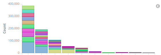 The next set of servers I looked at were the ones that host virtual machines. The above graph was supposed to show 11 host machines but one of them did not register even a single packet. Missing traffic basically means there has been no web traffic to that server at all, not even updates, which is alarming. Moreover, the traffic for these server were unusually lopsided. The uneven traffic distribution was a head scratcher. I expected all of them to have equal sized bars. After doing some research on high usage servers, I found couple of tools installed in those high usage machines, that required internet access. I was under impression that the host machines were hosting vms and nothing else but I stand to be corrected. I plan to move those services to virtual machines and keep the host machines as barebone as possible.
I built similar bar charts for the remaining servers and most of the traffic size were as expected. Domain controllers had high volume of traffic going to 8.8.8.8 but there were some instances where DNS lookup traffic was routing to Hawaiian tel server. I found one more server where all traffic to SAN network was going through firewall, due to some mysterious misconfiguration.
Finally, the most interesting traffic was seen in print server. Vendors have their monitoring tools installed in that virtual machine to monitor printer usage and refill toners as necessary. Almost 600k bytes have been sent to the vendor in last few weeks which is more that all but 3 of my server. Two of them are domain controllers and 99% of that traffic was dns lookup. While most of the traffic to the last server were being routed to SAN network.
After a birds eye view of the servers and digging into details when necessary, I have come to realization that few changes need to be made as soon as possible. The priorities are to correctly route SAN traffic for two server and talk to xerox about the amount of traffic they are collecting. It is time to remind them about possible HIPPA violation if the misuse this data and also determine type of data they are collecting. Moreover, I need better understand network traffic so I can do a deep inspection. While kibana has given me a great look into overall server traffic within my network, drilling down to details is a lot of query DSL using curl.
Printer dashboard
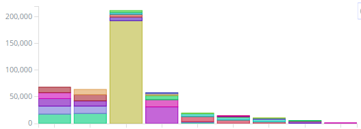
 After looking at the massive amount of data exfiltrating print server, I decided to look into individual printers. Some printers were sending data out individually, unrelated to print server traffic, as seen in the graph below. This graph represents data in three dimensions. X-axis represent the port number of traffic and y-axis has the external IP source and the total packet size. Each color block represents a printer. Out of 50 networked printer, about 15 were talking to external ip. Most of them were going to the printer manufacturer themselves. Xerox printers were sending data to xerox network and HP printers were sending data to HP ip ranges while the rest were from vpn users.
Total Traffic
 A time series graph depicting total traffic on a given day is another useful tool in my dashboard. The three lines in the graph red, blue and yellow represent 3 consecutive days. Blue represents traffic for that day and red represents the day before and yellow is total traffic from 48 hours hours ago. It is useful to compare total traffic of a given day to couple of days around it to get a sense of what is normal.
The above graph shows traffic is fairly consistent for most days. Weekends have low traffic as expected but there was one peak on 28th of November and the total traffic on that day is almost 3 time those of any other days.
 I zoomed into the graph to focus on traffic between 2pm and 3:30pm of November 29th which can be seen below. I chose 29th instead of the actual date of the traffic so I can compare 28th in red with 27th in yellow and 29th in blue. The total traffic exfiltrated on 28th is definitely alarming. However, I do not have expertise to understand what exactly happened in that time frame. I have reached out to few friends in the industry for help. As of now I have the data saved and I get go back to analyzing this day when I find someone or something with the expertise to do so.
Significant Terms
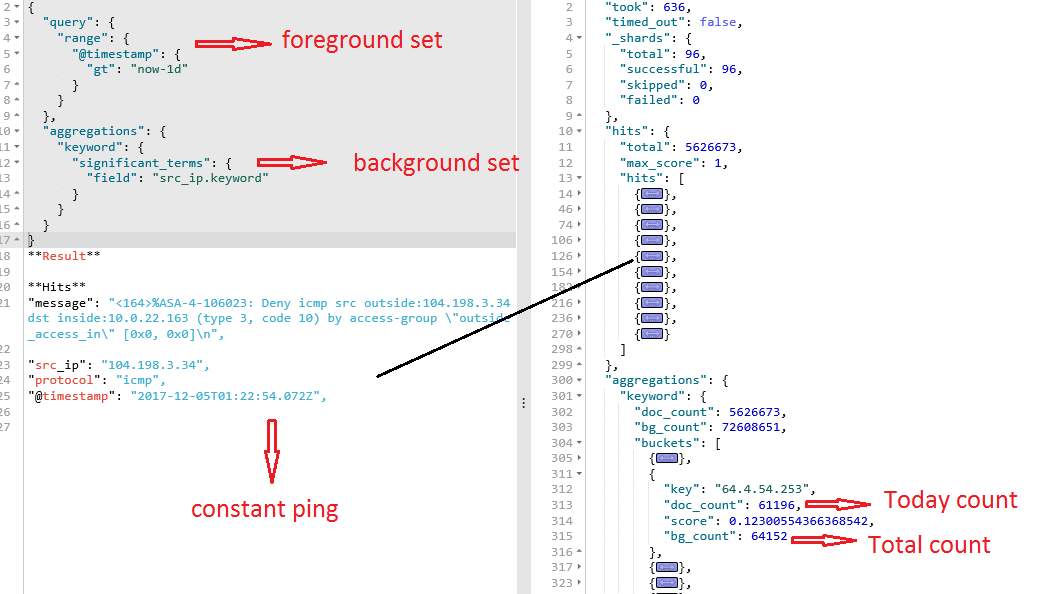 Elasticsearch has a great functionality of finding significant terms and it is fairly straight-forward to use. Significant terms calculates a score for all terms in foreground by comparing it to the documents in the background set. In the figure above, I defined foreground set as documents in the last 24 hours and background set as all documents in the collection. Within matter of seconds, elasticsearch was able to compare all documents in foreground and background set to give me a relative score. This score is not just a popularity contest, it is significant change in popularity between foreground and background set. There are option to boost certain fields as I learn more about network traffic in general
The result of significant term search above, ranked the unusually popular ip for that day 64.4.54.253. Out of 64 thousands documents in the whole collection, 61 thousand of them were from one particular day. It was the second most significant term for that day.
I am multiple significant term searches similar to the one above. One searches for VPN user and the ip they are logging in from. If the ip changes, it is possible that the user is using starbucks internet or their credential is possibly compromised. I have other searches defined to look for significant port numbers number for a given day. As a novice with limited understanding for internet traffic, I am very suspicious of traffic coming on unconventional ports.
Finally looking at the figure above, I see the results were pulled from documents that were spread out across 96 shards. As we know shards are lucene indexes and each elasticsearch is made up of one or more shard. I have two clusters of elastic, one for router traffic and the other for firewall. The router cluster did not get any hits, so all the traffic from this ip was going one or more of the routers I am not monitoring.
Even though the search was completed in the matter of seconds, as the number of shards in my firewall cluster grows, search will probably start slowing down. I will have to further divide firewall traffic into multiple cluster.
The possible partition, I can think of, are by month or traffic going to different sites or by ports. Firewall probably does not generate enough logs to justify clustering by month but the other two are viable options and I am torn between which one is the better option. I could combine smaller sites into one cluster and bigger sites as a separate one. If I chose to go this route, I could add router traffic into the respective clusters. On the other hand, separating traffic by port sounds interesting too. All DNS lookup can go into one cluster since it generates the most traffic. Similarly email and web traffic can have individual clusters and the rest of port can go into final cluster. The advantage of this configuration is the need to search in one cluster when I am digging into a particular type of traffic.
Actionable items
Collecting the data is fine, having dashboard is great, but it is all for naught if it does not give me actionable items. And fortunately ELK stack did direct me to lot of areas that need immediate or intermediate actions.
I have implemented few changes in the network since I started collecting these data. Printer data looks the most suspicious, so I changed the printer setting in all the printers generating traffic. I haven’t seen printer traffic in the last few days but disabling everything in the printer has hindered users from utilizing all the functionality in some printers which is creating extra work for already overworked IT team.
The second change I am working on is blocking ip that operate on unconventional ports. Granted some application may use those ports for legitimate reasons and I may block users from legitimate work related traffic. I have had few complaints after those changes but I have been resolved those issue as swiftly as I blocked them, unlike the printer issues which is still giving me headache. The interesting result from this massive blockage is, most of those ip are still restricted and no one seem to have noticed it.
The next step would probably be better segmentation of subnets. After I added router logs to the mix, I saw some traffic between two computers in different building that should not be talking to each other. I formatted both the computers with malware suspicion.
Finally, I need to better solution to analyze web and email traffic. I do not have expertise to understand web traffic nor do I have have knowledge to isolate suspicious email. Moreover, digging into individual suspicious traffic is not feasible. I need a better heuristics but that will only come with time and experience.
Conclusion
I have been using ELK stack for few weeks, I am really enjoying tweaking and testing to get better snapshot of traffic in my network. It gives me retrospective view of all the traffic which I never had before. I have been spending lot of my time at work with elastic and it has been fun. Elasticsearch is popular for its prowess when dealing with logs but it can do much much more. Elasticsearch can be used for any blob of text whether it is twitter or wikipedia. Logstash and Kibana might not be appropriate tool for those data sources but with python libraries, it is matter matter of writing scripts to load the data and pull it out of visualization. Elastic does the rest.
However, ELK stack has its limitations as a sole security tool. While it affords ability to replay traffic in case of intrusion, there is a need for real time intrusion detection system as well as ability to drill down into the nitty gritty. This is where bro and security onion comes in and apparently, they works very well with ELK and many organization deploy them together as their monitoring and security stack. The logs from firewall and routers are fed into bro which gives real time IDS with alerts. The data from bro is then loaded into ELK stack to get gives retrospective visuals. Finally, security onion opens up potential to drill down into dashboards generated by Kibana. Deploying and configure bro, elk and security onion is my goal for the next few months.